Introduction
As debate in Washington continues over how (or whether) to pay for the latest infrastructure plan, someone will inevitably claim it will pay for itself. (1) Such optimism reflects the belief that government spending creates jobs and grows the economy. If these positive effects were big enough, the additional taxes resulting from more workers and higher incomes would pay for the additional spending. Although government policy can affect the economy,(2) there is no credible evidence to suggest any major fiscal policy initiative – either taxes or spending – can ever fully pay for itself.
This issue brief examines the historical relationship between investment and economic growth and uses a simple economic model to illustrate why government infrastructure does not pay for itself. This result is due to a combination of factors, including the government investing in projects the private sector deems unprofitable, the crowding out effects of government spending, and the ongoing costs of maintenance and repair. There may be other compelling reasons to justify government investment, such as the provision of public services, but attaining the proverbial “free lunch” is not one of them.
Investment and Growth
Economic growth, measured in terms of the additional value of goods and services produced over time, is the result of the knowledge, skills, and abilities of workers (human capital) combined with the technology, tools, and resources available to help them do their job (physical capital).
The accumulation of physical capital over time results from the addition of new investment, minus the loss of old investment due to wear and tear, or technological obsolescence (a.k.a. economic depreciation). Historical data suggest more investment leads to faster economic growth, but not all investment is equally productive.
In the private sector, current investment decisions are primarily guided by the desire to meet the anticipated demand for future consumption. Businesses rely on prices determined by supply and demand to make investment decisions in anticipation of earning a profit. Higher profits encourage more investment, while losses deter further investment.
In the public sector, current investment decisions are often guided by political expediency, rather than economic efficiency. Politicians can be unduly influenced by public opinion polls and campaign contributions. That does not mean government investment is necessarily illegitimate or worthless. Indeed, major public-works projects like the interstate highway system undoubtedly provided a significant boost to the economy. But that does not mean a second interstate highway system would be as valuable as the first.
The problem with government investment is that it typically seeks to provide a public service that is not subject to the market discipline of profits and losses created through voluntary exchange. When the government builds a road, it does not rely on investors seeking to earn a profit by charging drivers a mileage-based user fee. Instead, the government builds a road with taxes or debt (which pays an interest rate unrelated to the success or failure of the road) while allowing drivers to use the road as much as they desire at no additional cost.
Government provision of public services can be justified on the grounds that market-based decisions do not always lead to the most socially desirable outcomes. But when investment decisions are not based on economics, the results are often disappointing from an economic perspective.
The Marginal Benefit of Additional Investment
The value of additional investment is a function of the cumulative amount of physical capital that already exists relative to the optimal amount. As previously noted, building the original interstate highway system provided a significant return on investment by reducing the cost of traveling and transporting goods across the country. But building additional roads, or maintaining existing ones, is unlikely to provide the same positive result.
To assess the marginal benefit of additional investment, the following regression analysis compares the statistical relationship between investment and real GDP per capita, using historical data from the Bureau of Economic Analysis (BEA).(3) The results indicate private investment is associated with higher growth, while government investment is associated with lower growth.
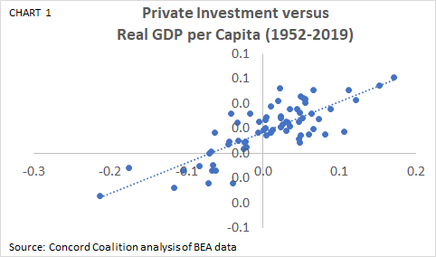
Chart 1 shows the annual change in private investment as a percent of GDP (X-axis), and the annual change in real GDP per capita (Y-axis).(4) The positive correlation suggests a 10 percent increase in private investment corresponds to a 2.8 percent increase in real GDP per capita. This relationship is the estimated short-run (annual) effect. The long-run (historical average) effect is estimated to be 0.8 percent.(5)
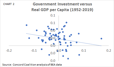
In contrast, Chart 2 shows there is a negative correlation between the annual change in government investment (X-axis) and the annual change in real GDP per capita (Y-axis).(6) The short and long-run effects are estimated to be -1.4 percent and -0.0 percent, respectively.
Recognizing government investment can enhance the value of private investment, (e.g. private goods transported on public roads), it is necessary to consider the possibility of such interactions. By including each type of investment separately in the regression analysis, the results indicate the short and long-run effects of private investment on real GDP per capita are 3.0 and 0.9 percent, respectively; and the short and long-run effects of government investment are slightly positive, but statistically insignificant.(7)
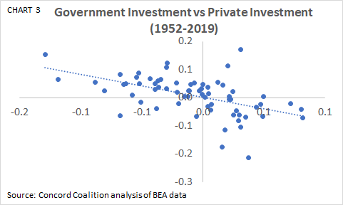
One possible explanation for this result is that even though government investment enhances private investment, it is less productive than private investment, and it reduces (or crowds-out) private investment. Chart 3 shows the negative short-run correlation between the annual change in government investment (X-axis) and the annual change in private investment (Y-axis). In the long-run, a 10 percent increase in government investment corresponds to -1.4 percent decrease in private investment.(8)
While correlation does not prove causation, these results suggest any bold claims that additional government investment will boost the economy enough to fully pay for itself should be taken with a grain of salt.
The Opportunity Cost of Government Spending
Conventional wisdom holds that rising levels of government debt reduce the amount of credit available to other borrowers and results in higher interest rates. Thus, government debt is said to “crowd out” other investment. But in a world of central banks, fiat currencies, and floating exchange rates, there is almost no limit to the supply of money. Higher demand does not lead to higher prices when supply is infinite. Although interest rates will eventually rise due to the inflation caused by too much money chasing too few goods, the arrival of higher prices may be delayed due to mitigating factors.(9)
Although the supply of money may be virtually infinite, the things money can buy at any given point in time are not. The production of goods and services typically involves a series of steps in which raw materials are transformed into intermediate goods which are transformed into finished products. For example, to make bread, we need to grow wheat. To grow wheat, we need to plow land. To plow land, we need tractors. To build tractors, we need plastic, steel, rubber, etc. Nearly every step of this process relies on trained individuals with unique skills and knowledge who utilize specific tools and material designed to meet their specialized needs.
Given the complex structure of production, an increase in the demand for bread cannot instantaneously bring about an increase in the supply of all the things needed to produce more bread. Likewise, a reduction in the demand for bread cannot instantaneously convert the people, places, and things previously used to produce bread into some other productive alternative.
At any given point in time, our economy is comprised of a specific set of goods and services, each with its own unique factors of supply and demand. When market conditions change – either because of fickle consumers, a financial crisis, or a global pandemic – some of the goods and services that existed before the change may no longer be suitable to meet the market conditions that exist after the change.
When workers are unemployed and productive resources are idled, it is often suggested that an increase in government spending can revive our economy. But government spending is rarely limited to unemployed workers and idled resources. More often, gainfully employed workers and fully utilized resources are diverted from one use or location to another (e.g. from building factories in Ohio to building schools in Texas). If this diversion is inconsistent with the changing market conditions, the result will be a misallocation of workers and resources, and fewer goods and services will be available in the desired quantities, relative to what would otherwise be available.(10)
Every dollar the government spends has a cost, regardless of whether the dollar comes from taxes, borrowing, or the printing press. When the government spends money, it diverts workers and resources from alternative uses. This form of crowding out is the opportunity cost of government spending.
A Simple Economic Model
To illustrate the potential economic impact of government investment on the economy, the following analysis uses a simple economic model in which the output of goods and services (Y) is determined by the input of technology, labor, and capital (A, L and K).(11) This model reflects long-run, supply-side effects, rather than short-run, demand-side effects.(12)
For purposes of this illustration, the model assumes the government spends $1 trillion on physical infrastructure (roads, transit, rail, power, water, communication, etc.) over eight years, funded entirely with government debt. Given the following assumptions: no crowding out of private investment; government and private investment are equally productive, and the elasticity of labor is 0.2 percent;(13) by the end of the eight-year period, the stock of physical capital would be 1 percent higher, real GDP would be 0.5 percent higher, and total hours worked would be 0.1 percent higher, or roughly 132,000 full-time equivalent (FTE) jobs.(14)
Despite these favorable assumptions, the $1 trillion investment would not produce enough economic growth to fully pay for itself because maintaining the economic value of the investment over time would require continued maintenance and repairs.(15) As a result, the nominal amount of debt incurred to fund the investment would grow indefinitely. Whether the debt increases or decreases as a share of GDP depends on the size of the primary deficit (total deficit minus net interest), the nominal interest rate relative to the nominal GDP growth rate, and total government debt as a share of GDP. Although these factors exceed the scope of this analysis, current trends do not look promising.
Conclusion
Both economic theory and common sense suggest government investment can potentially enhance the value of private investment and boost economic growth. But that does not mean more government investment is always better. Indeed, empirical analysis suggests the marginal economic impact of additional government investment is either negative or indistinguishable from zero. Moreover, a simple economic model that assumes government investment is just as productive as private investment shows the additional economic growth would not fully pay for the investment after accounting for the cost of economic depreciation.
This evidence presents a challenge to policymakers seeking to enact a major infrastructure plan. Do they follow the path of least resistance and add the cost to the national debt, or do they make the hard choices and actually pay for it? Whatever they decide, they should not expect to settle in for a sumptuous free lunch.
[1] Infrastructure investment pays for itself | TheHill
[2] Dynamic Analysis | Congressional Budget Office (cbo.gov)
[3] https://apps.bea.gov/iTable/index_nipa.cfm
[4] Gross private domestic fixed investment in residential and nonresidential structures, equipment, intellectual property, and software.
[5] The regression is estimated in natural logs as: RealGDP/Population(t) = RealGDP/Population(t-1) + PvtInvestment/GDP(t) + PvtInvestment/GDP(t-1), where the investment coefficient at time (t) is the short-run effect and the sum of the investment coefficients at time (t) and (t-1) is the long-run effect.
[6] Gross government investment (both defense and nondefense) in structures, equipment, intellectual property and software at the federal, state and local level.
[7] RealGDP/Population(t) = RealGDP/Population(t-1) + PvtInvestment/GDP(t) + PvtInvestment/GDP(t-1) + GvtInvestment/GDP(t) + GvtInvestment/GDP(t-1), where the lagged dependent variable serves as a proxy for the other omitted variables that also contribute to economic growth.
[8] PvtInvestment/GDP(t) = PvtInvestment/GDP(t-1) + GvtInvestment/GDP(t) + GvtInvestment/GDP(t-1)
[9] Price*Quantity=Money*Velocity, or PQ=MV, therefore P=MV/Q
[10] Economics after the Virus | National Affairs
[11] Y=A*L^(a)*K^(1-a), where (a) is the labor share of income, (1-a) is the capital share of income, and 0<a<1. The technology term A, or total factor productivity, is a statistical residual that reflects the additional output that cannot be attributed to either labor or capital due to measurement error.
[12] How CBO Analyzes the Effects of Changes in Federal Fiscal Policies on the Economy
[13] LaborSupply&FiscalPolicy.fm (cbo.gov)
[14] Labor Force Characteristics (CPS) (bls.gov); FTE = (35 hours)*(52 weeks)
[15] Measuring Infrastructure in the Bureau of Economic Analysis National Economic Accounts | U.S. Bureau of Economic Analysis (BEA); Assuming an average depreciation rate of 2 percent.
Continue Reading