Download the pdf: History and Future of the Social Security Trust Fund_ Part II
Introduction
Part II of this issue brief series explains how changes to the Social Security benefit formula in the 1970s eliminated the possibility of relying on economic growth to reduce the long-run deficits resulting from demographic change, and how these changes revived the trust fund controversy described in Part I.
When Social Security was enacted in 1935, it provided a fixed level of benefits that changed only when Congress enacted an ad hoc adjustment. This process allowed Congress to periodically increase benefits on a one-time basis without committing to additional increases in the future. However, in 1972, under the guise of providing automatic cost-of-living adjustments (COLAs), Congress enacted a new benefit formula. This formula replaced the ad hoc process with an automatic annual increase. This shift represented a fundamental change in the nature of the Social Security program.
By increasing benefits automatically, the new formula meant that the program could no longer rely on future economic growth to reduce the cost of a fixed level of benefits relative to a rising level of wages. When adverse economic conditions exposed a flaw in the formula and falling birth rates revealed the projected cost of the formula was higher than expected, Congress faced a dilemma – should it renege on the promise of automatic benefit increases or enact higher payroll taxes?
In 1977, Congress chose the path of least political resistance, fixing the flaw in the formula while maintaining the automatic increases, but refusing to impose the payroll taxes needed to fund them. When Congress was forced to address a temporary funding short-fall in 1983, it inadvertently resurrected the trust fund controversy.
From Static to Dynamic Assumptions[1]
As explained in Part I of this series, opposition to building up an enormous trust fund balance led Congress to delay scheduled payroll tax increases as well as enact higher benefits. These changes were possible because benefits remained fixed after each ad hoc increase, whereas wages continued to grow due to inflation and productivity. Higher wages produced the additional payroll tax revenue needed to offset the lower payroll tax rates and the higher benefit payments.
Even though Congress enacted periodic benefit increases throughout the 1950s and 1960s, there was growing interest in providing automatic cost-of-living adjustments. However, there was a significant impediment to doing so. Since 1935, the actuaries who prepared long-range cost estimates for Social Security had utilized an actuarial technique known as the level-earnings assumption.
Basically, the actuaries assumed wages and prices would remain frozen at their current level forever into the future. That’s equivalent to assuming wages and benefits grow at the same rate (i.e., zero). In 1935, the level-earnings assumption did not seem unreasonable. Indeed, average wages were still below the level that prevailed in 1920 (see Part I Figure 6). The actuaries believed this assumption imposed a measure of fiscal discipline and provided a cushion against unanticipated events.
Congress was willing to go along because, as time passed and wages grew, it was able to periodically dispense the revenue windfall in the form of higher benefits. Despite the recurring availability of these windfalls, critics began to suggest a new approach was needed. They pointed out rising inflation imposed an undue burden on Social Security beneficiaries who were forced to wait for Congress to enact a benefit increase. Their proposed solution was an automatic cost-of-living adjustment based on the annual change in consumer prices (i.e., inflation rate).
The idea of indexing benefits to prices (price-indexing), or even wages (wage-indexing), had been contemplated for years.[2] But the implementation of an automatic benefit increase was incompatible with the level-earnings assumption. Any long-run projection based on level wages and rising benefits would show large and growing deficits. Critics began a campaign to discredit the level-earnings assumption and urge the adoption of dynamic assumptions. This campaign led to the 1971 Advisory Council recommendation that long-run projections should assume wages will rise in the future.[3]
By adopting dynamic assumptions, Social Security suddenly appeared to have a significant surplus. But it’s important to understand the source of the surplus. As noted above, under static assumptions, wages and benefits were both frozen at their current level. Under dynamic assumptions, wages are assumed to grow due to inflation and productivity, but benefits are assumed to remain frozen until Congress votes to increase them. Thus, the newly created surplus reflected the difference between the additional payroll taxes generated by the projection of rising wages and the cost of frozen benefits.
Unlike a revenue windfall that results from an actual wage increase, the surplus under dynamic assumptions was merely assumed. Nevertheless, members of Congress seized on the Council’s recommendation and urged an immediate 20 percent across-the-board increase, followed by automatic cost-of-living increases thereafter.[4] Bypassing the regular committee process, an indexing amendment was offered on the Senate floor to a bill increasing the statutory debt limit. It passed overwhelmingly and was signed into law in July of 1972.[5]
The congressional debate that preceded passage of the indexing amendment focused on keeping benefits up with inflation.[6] For those already receiving benefits, the amendment produced the intended result. Benefits increased with the rise in consumer prices. However, for those not yet receiving benefits, the result was entirely different. Depending on the annual rate of change in wages and prices, the initial benefit for those who became newly eligible would either rise, fall, or remain the same relative to their previous wages. This erratic variation was the unintended result of using the same benefit formula for both current and future beneficiaries.[7]
For retired workers, whose wages were fixed because they were no longer working, increasing the formula by the rate of inflation would increase their benefits by the same amount. But for current workers, whose wages were generally rising due to inflation and productivity, increasing the formula by the rate of inflation would change their initial benefit at retirement by different amounts, depending on the relative change in wages and prices, and where their wages fell within the progressive benefit formula.
Figure 1 shows how benefits would have varied under the 1972 formula based on alternative assumptions about the rate of inflation (CPI) and the growth in average monthly earnings (AME). Initial benefits paid in the year of retirement are shown as a percentage of the wages earned in the year prior to retirement. This percentage is one of several ways to measure “replacement rates,” as discussed below. For hypothetical workers who always earned the average wage and retired at age 65, replacement rates could range from 37 to 79 percent in 2052, compared to 42 percent in 1972. For workers earning half the average wage, replacement rates could range from 54 to 130 percent in 2052, compared to 56 percent in 1972.[8]
Figure 1: Replacement Rates at Age 65 under Alternative Assumptions (1972 and 2052)
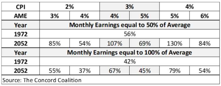
In the 1972 and 1973 Trustees’ reports, wages were assumed to grow at 5 percent and inflation at 2.75 percent. Under these assumptions, replacement rates would remain roughly constant.[9] But if these two assumptions were changed in either direction, then replacement rates would either rise or fall, in some cases dramatically.[10] The potential variation in initial benefit replacement rates might have gone unnoticed for years, but changing economic and demographic assumptions quickly revealed the flaw.[11]
The 1972 amendment was based on two key assumptions: that wages would rise nearly twice as fast as inflation, and the total fertility rate would remain near the baby-boom level. Under these assumptions, initial benefits would rise in line with wages, and there would be plenty of workers to support each beneficiary, without raising the payroll tax much beyond the 11.7 percent rate scheduled to take effect in 2011. However, the decade of the 1970s saw rising inflation and the end of the baby boom. The flawed formula caused benefits to rise faster than wages and falling birth rates resulted in a declining ratio of workers-to-beneficiaries. As a result, the Trustees began to report rising deficits.
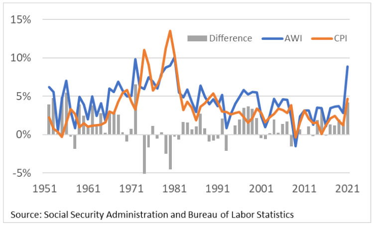
Historically, the growth in average wages tends to exceed the growth in consumer prices. Higher wages provide additional payroll taxes to fund annual cost-of-living adjustments (COLAs) for current beneficiaries. However, during the stagflation period from the mid-1970s to early-1980s, inflation often exceeded wages, resulting in negative real (inflation-adjusted) average wage growth. Figure 2 shows the change in wages, based on the average wage index (AWI), and the change in prices, based on the consumer price index (CPI). The difference between them is the real wage differential (AWI-CPI).
Figure 2: Average Annual Change in Wages (AWI) and Prices (CPI)
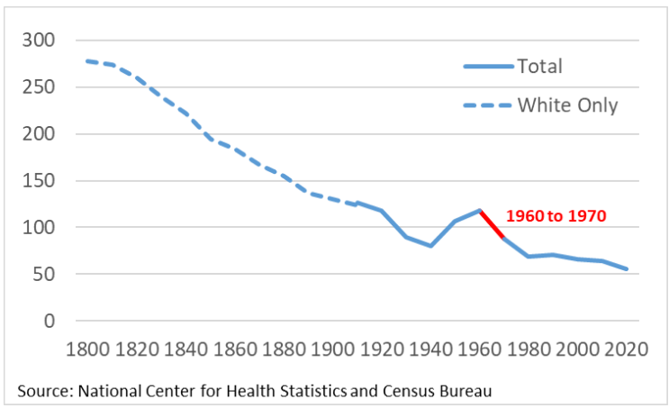
The other factor that contributed to the declining financial outlook of the Social Security program was the end of the baby boom.[12] Historically, birth rates had been on a steady decline, temporarily interrupted by the baby boom (1946-1964).[13] Despite every indication the decline had resumed by 1970 (Figure 3), the cost estimates used in the 1972 and 1973 trustees’ reports assumed the total fertility rate would average 2.5 births per woman over her lifetime.[14]
Figure 3: Number of Births per 1,000 Women 15-44 Years Old
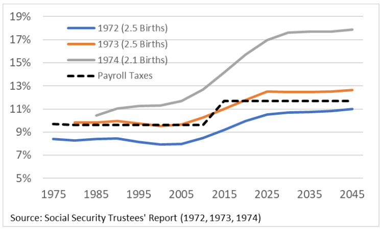
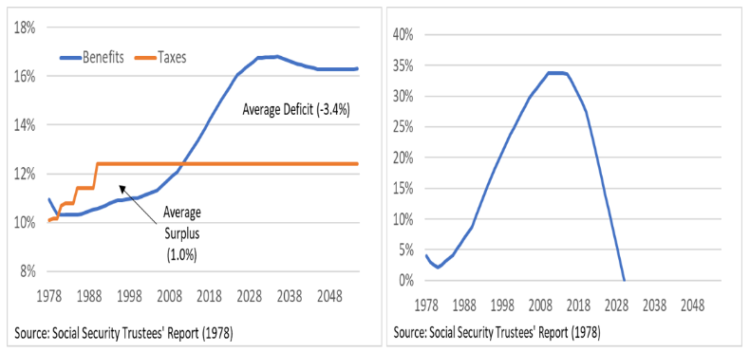
When the Trustees updated their economic and demographic assumptions in 1974, the results showed a significant increase in the long-run deficit. Figure 4 shows the projected cost of Social Security benefits as a percentage of taxable payroll, before and after the 1972 amendments, assuming a total fertility rate of 2.5 births per woman and average wage growth of 5.0 percent and 2.75 percent inflation. In 1974, when the trustees lowered the fertility rate to 2.1 births and increased the inflation rate to 3.0 percent, which reduced the real wage differential, the long-term cost increased dramatically.[15]
Figure 4: Social Security Taxes and Benefits as Percent of Taxable Payroll
In response to these rising costs, the Senate Finance Committee and the House Ways and Means Committee requested the appointment of an independent consultant panel to examine the problem and develop alternatives. The panel issued its report in 1976 and recommended that Congress index initial benefits to prices, rather than wages.[16] But advocates for higher benefits sought to replace the flawed 1972 formula with another wage-indexing formula that was less erratic and unpredictable.
Ironically, the flaw of the 1972 formula became its biggest asset. Between 1973 and 1977, the projected cost more than doubled from less than 13 percent to more than 26 percent of taxable payroll. Advocates of wage-indexing sought to portray their version of wage-indexing as a significant savings because it would “only” cost 16 percent of taxable wages.[17]
Advocates of wage-indexing persuaded Congress to adopt their plan in 1977 by simultaneously arguing that it was cheaper than current law and more generous than price-indexing. The fact that lower wages, higher inflation, and declining fertility had rendered wage-indexing unaffordable at the scheduled payroll tax rate did not seem to matter. Advocates dismissed the projections of future deficits by suggesting economic and demographic changes might solve the problem. If not, Congress could encourage the elderly to work longer and re-authorize the use of general revenue, or so they suggested.[18]
Figure 5 shows the projected short-run surpluses were insufficient to offset the projected long-run deficits, and thus the 1977 amendments failed to maintain trust fund solvency throughout the projection period.
Figure 5: Social Security Taxes, Benefits, and Trust Fund Balance (Percent of Taxable Payroll)
By refusing to adopt the more affordable price-indexing alternative, or schedule the future payroll taxes increases needed to fund wage-indexed benefits, Congress ignored the admonition given to them by the 1976 Consultants Panel: “This Panel gravely doubts the fairness and wisdom of now promising benefits at such a level that we must commit our sons and daughters to a higher tax rate than we ourselves are willing to pay.”[19]
Replacement Rates and Demographic Change
The adverse impact of the 1972 and 1977 amendments on the financial condition of the Social Security program cannot be overstated. To understand this impact, it’s necessary to review the concept of replacement rates and consider how they interact with demographics. Replacement rates measure the ratio of benefits to wages – or how much of a worker’s earnings are replaced by Social Security benefits in retirement. Demographics determine the ratio of workers-to-beneficiaries – or how many workers are available to pay the taxes needed to support each beneficiary, although this ratio is somewhat amenable to changes in the retirement age.
Replacement rates provide an individual level measure that reflects the initial benefit paid to an individual in the year of retirement divided by the wages earned by the same individual in the year (or years) prior to retirement. A closely related measure, which we will call the “average cost rate,” provides an aggregate level measure that reflects the average benefit paid to all beneficiaries in any given year divided by the average taxable wage earned by all workers in that same year. If wages and prices remained constant over time, the weighted average replacement rate and the average cost rate would be the same, ignoring the effects of differential mortality.[20]
The financial impact of these interactions can be illustrated with the formula: t = (b/w) / (W/B), where (t) is the payroll tax rate needed to fund benefits on a “pay-as-you-go” basis; (b/w) is the ratio of benefits-to-wages, which reflects the average cost rate; and (W/B) is the ratio of workers-to-beneficiaries, which reflects demographic change. For example, if the average benefit equals 40 percent of the average taxable wage, and there are four workers per beneficiary, then the payroll tax would need to be 10 percent (40%/4). If the W/B ratio falls to 3-to-1, or 2-to-1 as projected to occur with lower birth rates, then the payroll tax rate would need to be 13 percent (40%/3), or 20 percent (40%/2).
Figure 6: Ratio of Workers-to-Beneficiaries Determines Cost of Benefits

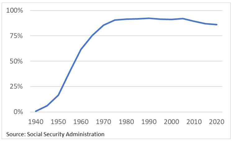
During the early years of the program, the ratio of workers-to-beneficiaries was higher because most of the elderly were ineligible for benefits. They were ineligible because Social Security did not exist when they were younger, so they did not contribute to the program. As Figure 7 shows, the share of elderly receiving Social Security benefits did not reach 90 percent until the early 1970s.[21] The slight decline in recent years is largely due to the increase in the full retirement age (FRA), which reduces monthly benefits for those who retire at an earlier age.[22]
Figure 7: Percentage of Elderly (Age 65+) Receiving Social Security Benefits
As noted above, the Social Security benefit formula was designed to be progressive. That means the formula provides higher replacement rates for lower-wage workers, and lower replacement rates for higher-wage workers. Replacement rates have varied over the years based on changes in the benefit formula, changes in the distribution of wages subject to the payroll rate, and the difference between average wage growth and the increase in consumer prices.
Figure 8 compares initial replacement rates to average cost rates. The blue line reflects the initial replacement rate at age 65 for hypothetical average wage workers.[23] The orange line reflects the average cost rate for all beneficiaries (retired, disabled, spouses and survivors), regardless of their level of wages or initial year of eligibility.[24]
Replacement rates in 1940 (when monthly benefits were first paid) averaged less than 25 percent. As wages grew and benefits remained frozen until 1950, replacement rates fell to roughly 15 percent. Between 1950 and 1970, replacement rates stabilized between roughly 25 and 30 percent due to a series of ad hoc benefit increases. The 1972 amendments allowed replacement rates to rise above 50 percent until the 1977 amendments reduced them back to 40 percent where they roughly stabilized and the average cost rate began to converge.
The average cost rate generally lagged behind the initial replacement rate. The decline in the average cost rate between 1965 and 1970 was due to increases in the maximum taxable wage which increased the denominator more than the numerator.[25]
Figure 8: Initial Replacement Rates and Average Cost Rates
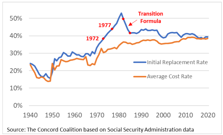
Replacement rates can be misleading and incomplete, as The Concord Coalition has previously written.[26] But they can also illustrate how changes in the benefit formula for newly eligible beneficiaries would, if left unchanged, eventually change the average cost rate for the entire program. Although everyone received a 20 percent benefit increase in 1972, initial replacement rates began to rise dramatically thereafter. The longer initial rates are allowed to rise, the more costly the program becomes as newer beneficiaries with higher benefits replace older beneficiaries with lower benefits through the process of attrition.
The 1972 formula continued to increase replacement rates even after Congress enacted the 1977 formula due to its delayed implementation. The 1977 formula was first applied to those who turned age 62 in 1979, and those born from 1917 through 1921 were provided a special transition formula.[27] These birth cohorts were known as “notch babies” due to the (erroneous) belief they were treated unfairly relative to those born both before and after.[28]
The 1977 amendments changed the 1972 formula by providing a separate formula for newly eligible beneficiaries versus those already receiving benefits. This formula was designed to provide roughly constant initial replacement rates, while still maintaining cost-of-living adjustments for existing beneficiaries.[29]
Despite stabilizing initial replacement rates at roughly 40 percent for hypothetical average wage workers retiring at the FRA, the Social Security program still faced a significant long-run shortfall due to changing demographics. Even though Congress had scheduled to increase the payroll tax rate to 12.4 percent in 1990, that was not enough to balance the program over the 75-year projection period. The 1978 Trustees report showed the Social Security trust fund would be depleted in 2028. The continuation of adverse economic conditions accelerated the depletion date to 1983. As a result, Congress was soon forced to consider additional changes.
The Greenspan Commission
As the Social Security program entered the decade of its 50th anniversary, the inflation rate continued to equal or exceed average wage growth and the trust fund was shrinking rapidly. By 1981, the Trustees projected insolvency by 1983 or 1984 under all but the most optimistic assumptions.[30] President Reagan established the National Commission on Social Security Reform to “identify problems… and provide appropriate recommendations.”[31] Alan Greenspan, who later served as Chairman of the Federal Reserve, was the Commission’s Chairman, hence it became known as the “Greenspan Commission.”
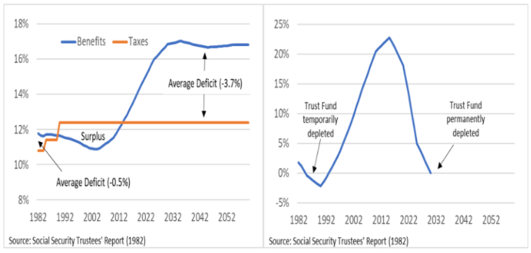
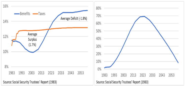
The most critical problem facing the Commission was the imminent, but temporary, insolvency of the trust fund. As noted above, the 1977 amendments had scheduled to increase the payroll tax rate to 12.4 percent in 1990. Once the higher rate took effect, the program was projected to run annual surpluses again until 2010 and assuming the trust fund had borrowing authority, it would have returned to a positive balance by 1994 and remained solvent through 2030.[32]
Figure 9: Social Security Taxes, Benefits and Trust Fund Balance (Percent of Taxable Payroll)
The Commission’s recommendations primarily focused on addressing the immediate shortfall. The most significant changes included delaying annual COLAs from June to December; taxing up to 50 percent of Social Security benefits for higher-income beneficiaries; covering newly hired federal employees and nonprofit employees; requiring the self-employed to pay the same payroll tax rate as other workers; increasing the payroll tax rate 0.6 percent in 1984 and 0.72 percent in 1988 and 1989; and making intragovernmental transfers based on noncontributory military wages credits.[33] These transfers are explained in Part III of this series.
The Commission was unable to reach consensus on how to eliminate the entire 75-year actuarial deficit. They were divided between raising the retirement age and increasing the payroll tax rate. When the legislation was considered by the House of Representatives two amendments were offered to address the remaining shortfall: an amendment to raise the full retirement age from 65 to 67 over the period 2000 to 2022; and an amendment to increase the payroll tax from 12.4 to 13.46 in 2010. The first amendment passed (228-202), and the second amendment failed (132-296).[34]
Following enactment of the 1983 amendments, the Trustees reported cash-flow surpluses were restored through 2020 and the trust fund would remain solvent throughout the 2050s.[35]
Figure 10: Social Security Taxes, Benefits, and Trust Fund Balance (Percent of Taxable Payroll)
Neither the Greenspan Commission nor the Congress ever publicly debated the prospect and implications of building up and drawing down an enormous trust fund balance.[36] Nevertheless, this roller coaster effect was the inevitable consequence of achieving 75-year actuarial balance, as explained in Part III of this series. The 1983 amendments thus led to a return of the trust fund controversy as policymakers found themselves with a growing Social Security surplus, but no agreement on what to do with it.
Conclusion
Prior to enactment of the 1972 amendments, Social Security benefits remained fixed unless Congress voted to change them. Fixed benefits provided the program with an economic safety-net because rising wages would generate additional payroll taxes allowing the program to grow its way out of almost any foreseeable financial problem. When Congress enacted automatic benefit increases based on the annual growth in wages and prices for initial and subsequent benefits, respectively, it eliminated this safety-net. The future financial viability of the program became almost entirely dependent upon demographics.
The end of the baby-boom led to a projected decline in the future ratio of workers-to-beneficiaries, resulting in rising long-run deficits. These deficits were compounded by a flaw in the 1972 formula. Congress fixed the flaw in 1977, while essentially ignoring the long-run deficits. When Congress was forced to address a temporary funding shortfall in 1983, it only partially addressed the long-run deficits, thus inadvertently resurrecting the trust fund controversy. Part III of this series explains why the public is understandably skeptical about the merits of investing surplus payroll taxes in government securities, and considers the lessons policymakers should learn from this controversy.
[1] Policymaking for Social Security | (brookings.edu) Chapters 17-19.
[2] Policy Issues in Social Security | (ssa.gov)
[3] 1971 Advisory Council | HathiTrust Digital Library
[4] Cost-of-Living Adjustment | (ssa.gov) The original COLA provision only applied when inflation exceeded 3 percent, but this requirement was eliminated in 1986.
[5] Social Security history | (ssa.gov)
[6] Social Security Amendments of 1977 Vol 3.pdf | (ssa.gov) (WMCP 95-48) It’s unclear whether Congress knew the 1972 amendments were expected to result in a two-tiered system in which initial benefits for newly eligible beneficiaries would increase with wages, whereas subsequent benefits paid in the following years would increase with prices. In 1977, the House Ways and Means Committee noted: “It can be argued that Congress intended that replacement rates should remain constant at the levels established by the 1972 amendments which provided for automatically increasing benefits as the cost of living rises. It can also be argued that Congress did not endorse constant replacement rates at that time but merely wished to keep benefits up with increases in the cost of living.”
[7] An analysis of the factors determining benefits | HathiTrust Digital Library
[8] These calculations include real wage differentials (AME-CPI) of 1 and 2 percent, rather than 2 to 2 ½ percent as projected by the Social Security Administration (see note #9 below).
[10] Financing Social Security: Issues for the Short and Long Term | (cbo.gov) Table 10
[11] 1975 Advisory Council | HathiTrust Digital Library
[12] By 2030, All Baby Boomers Will Be Age 65 or Older | (census.gov)
[13] 1-11-b-vital stat.pdf | (census.gov); Table 1-1. Live Births, Birth Rates, and Fertility Rates, by Race: United States, 1909-2003 | (cdc.gov); NVSS – Birth Data | (cdc.gov)
[14] 1973TR.pdf | (ssa.gov); note038.pdf | (ssa.gov)
[16] Social Security History | (ssa.gov)
[17] 1977TR.pdf (ssa.gov); 1978TR.pdf | (ssa.gov)
[18] Social Security Financing Proposals: Hearings Before Senate Subcommittee on Social Security | Google Books Testimony of Robert Ball, former Commissioner of Social Security
[19] Social Security History | (ssa.gov)
[20] The Empirical Relationship Between Lifetime Earnings and Mortality (cbo.gov)
[21] Annual Statistical Supplement, 2022 – Interprogram Data (3.C) | (ssa.gov)
[22] Normal retirement age (NRA) | (ssa.gov)
[24] Annual Statistical Supplement, 2022 – OASDI Covered Workers (4.B) | (ssa.gov); Annual Statistical Supplement, 2022 – Summary of OASDI Benefits in Current-Payment Status (5.A) | (ssa.gov)
[25] Contribution and Benefit Base | (ssa.gov)
[26] Social Security Replacement Rates: “Nudging” in the Wrong Direction? – The Concord Coalition
[27] The Notch Factsheet | (ssa.gov); Computing a Social Security benefit after the 1977 amendments | (ssa.gov)
[28] Social Security History | (ssa.gov); Social Security: The Notch Issue | (congress.gov)
[29] Social Security Replacement Rates: “Nudging” in the Wrong Direction? – The Concord Coalition See Appendix for explanation of current formula
[30] 1981TR.pdf | (ssa.gov) Table 14 combined OASDI trust funds
[31] Social Security History | (ssa.gov)
[33] Social Security Amendments of 1983: Legislative History and Summary of Provisions (ssa.gov)
[34] Social Security Amendments of 1983: Legislative History and Summary of Provisions (ssa.gov)
[36] hrg100-812.pdf (senate.gov); Testimony of Robert Myers, former Social Security Chief Actuary and Executive Director of the Greenspan Commission
Continue Reading